Tested on Ubuntu 18.04 and Windows 7/10
Products
Resources
Contact Us
About Us
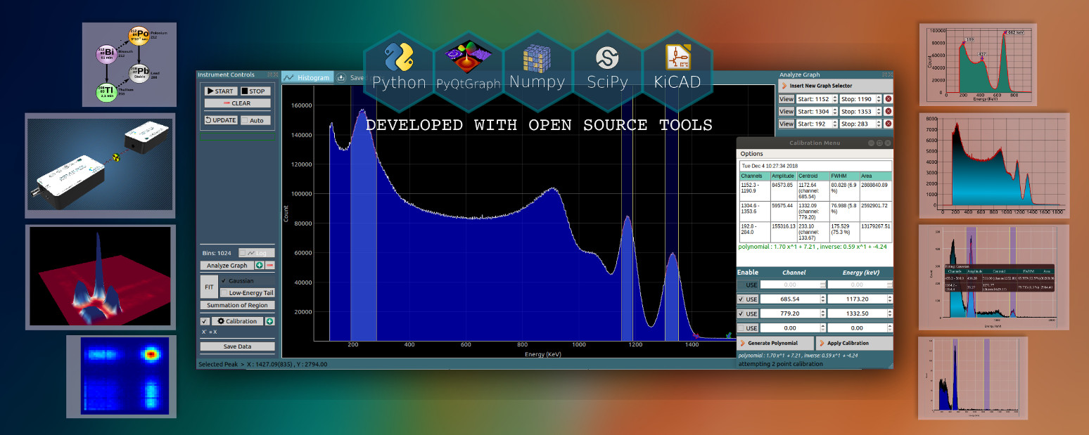
Compatible with our Multi Channel analyzers, Alpha Spectrometers, and Gamma Spectrometers
Analysis -> multi-point calibration, Gaussian Fitting, Low-Energy tail fitting, summation
Offline Data analysis of csv files
LGPL licensed source code supplied free with the instrument
Standalone Python library for acquisition and analysis.
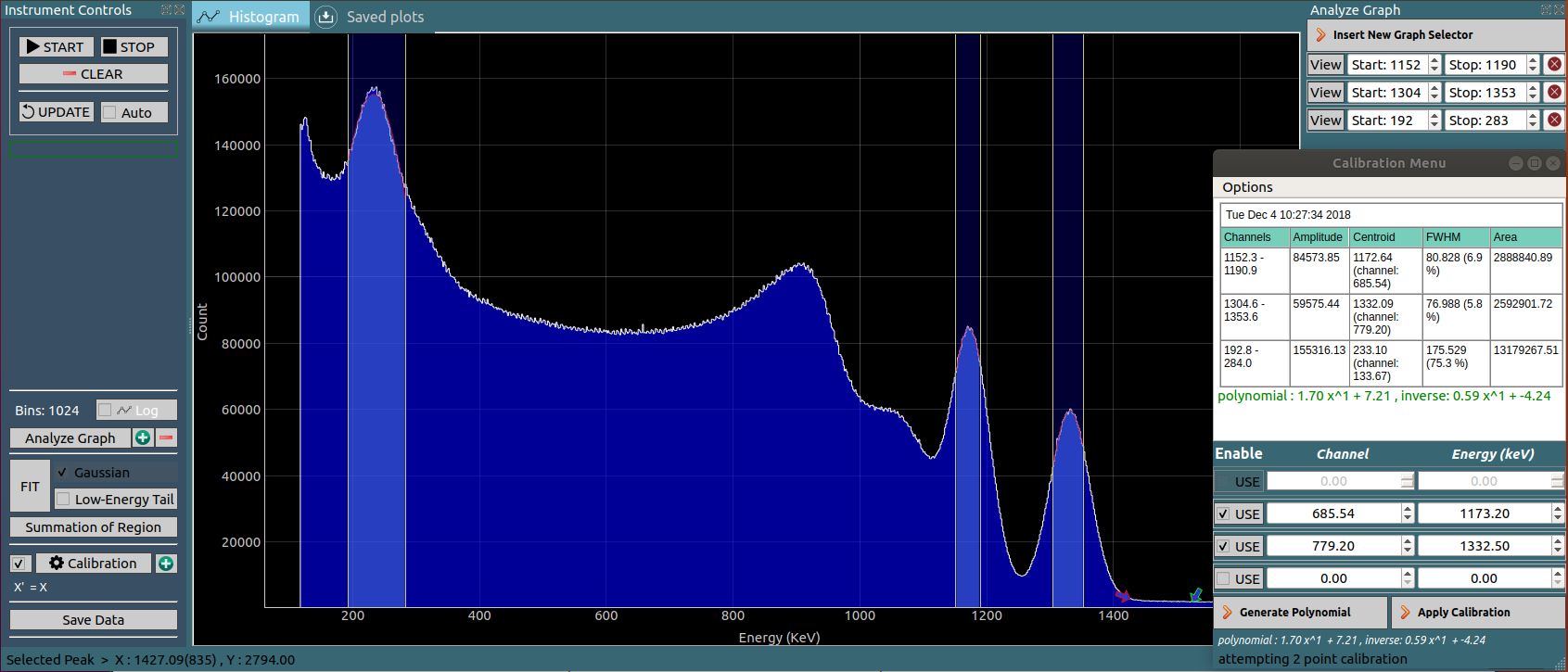
This tutorial explains how to use the region selectors for calculating centroids through gaussian fitting, and using the values to calibrate the instrument.
CNSPEC version > 6.0.0 must be installed. Or download the library : MCALib.py, and make sure the following packages are installed
Create a new python file. In case you downloaded MCALib.py , it must be located in the same directory.
import time,sys
from MCALib import connect

device = connect(autoscan = True) # automatically detect the hardware
#device = connect(port = '/dev/ttyUSB0')  #Search on specified port
if not device.connected:
	print("device not found")
	sys.exit(0)
print("Device Version",device.version,device.portname) #Display the version number

device.startHistogram()  #start data acquisition
time.sleep(5) # Wait for 5 seconds for gather some events.
device.sync() # fetch data from the hardware
x = device.getHistogram()  # Array of counts

from matplotlib import pyplot as plt
plt.plot(x)
plt.show()
Create a new python file. In case you downloaded MCALib.py , it must be located in the same directory.
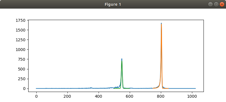
The results of the above code on offline analysis of 212-Bismuth spectrum are shown
Gaussian fitting was carried out on the first peak(Green) and overlaid.
Gaussian+Low energy tail(Lorentzian) was carried out on the second peak (Orange).

import time,sys
import numpy as np
from MCALib import connect

dev = connect()  # 'dev' contains a range of methods for acquisition and analysis
fname = 'bi212.csv'  #Supply your filename here.
dev.loadFile(fname)
# Get the data. Supply an optional name argument in case of multiple files/connected hardware.
x = dev.getHistogram() #name = fname / name='/dev/ttyUSB0'
np.set_printoptions(threshold = np.inf,precision = 0,suppress=True) #print the whole array. No decimal Points. Suppress scientific notation
print (x)
import matplotlib.pyplot as plt
plt.plot(x) #Plot RAW data
FIT = dev.gaussianFit([500,600]) #Apply a gaussian FIT between 500 and 600 channel.
if FIT: #If fit was successful
	plt.plot(FIT['X'],FIT['Y']) #Plot fitted data
	print('Gaussian Fit : ',FIT['centroid'],FIT['fwhm'])
FIT = dev.gaussianTailFit([750,850]) #Apply a gaussian+Lorentzian FIT between 700 and 900 channel.
if FIT:
	plt.plot(FIT['X'],FIT['Y']) #Plot fitted data
	print('Gaussian+low energy tail Fit : ',FIT['centroid'],FIT['fwhm'])
plt.show()
We are in the process of implementing a flow based approach for numerical analysis. A video is shown below.
List mode data can be passed through which are basically operators for binning/analysis/fitting etc, and can be further attached to visualization blocks such as 2D and 3D histograms.
Although the same can be achieved with 10 lines of Python code, this approach might come in handy for demonstrating the flow of logic for processing data. There is a long way to go, and we have also envisioned energy gates for processing multi parameter list mode data.