Multi-Channel Analyzers sort gaussian pulses into channels based on their pulse heights, in order to generate a spectrum. Our compact, USB powered MCAs and accompanying cross-platform, open-source software enables easy visualization and analysis of pulse outputs from various spectrometers.
Software link3.3V Shaped Input. 3uS rise time.
12-bit adjustable threshold
12-bit ADC
1024 channels. Fully USB powered unit
16 million counts per channel
8uS processing time per pulse
Fully featured Python software supplied open-source.

4V Shaped Input. 3uS rise time.
12-bit adjustable threshold
16-bit ADC
4096 channels. Fully USB powered unit
2 Bytes per channel.
10uS processing time per pulse including 3uS rise time
Fully featured Python software supplied open-source.

import time,sys
import numpy as np
from MCALib import connect

dev = connect()

fname = 'DATA/bi212_19mA_10min_31mar18/data_240mins.csv'
dev.loadFile(fname)

# Get the data. Supply an optional name argument in case of multiple files/connected hardware.
x = dev.getHistogram() #name = fname / name='/dev/ttyUSB0'

#Optional-Uncomment next two lines to print the whole array. No decimal Points. Suppress scientific notation
#np.set_printoptions(threshold = np.inf,precision = 0,suppress=True) #
#print (x)

#plot the loaded spectrum
import matplotlib.pyplot as plt
plt.plot(x) #Plot RAW data

FIT = dev.gaussianTailFit([750,850]) #Apply a gaussian+Lorentzian FIT between 700 and 900  channel, and overlay it.
if FIT:
	plt.plot(FIT['X'],FIT['Y']) #Plot fitted data
	print('Gaussian+low energy tail Fit : ',FIT['centroid'],FIT['fwhm'])

FIT = dev.gaussianFit([500,600]) #Apply a gaussian FIT between 500 and 600 channel.
if FIT:
	plt.plot(FIT['X'],FIT['Y']) #Plot fitted data
	print('Gaussian Fit : ',FIT['centroid'],FIT['fwhm'])

plt.show()
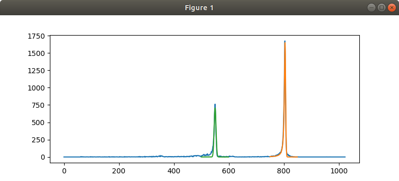
The results of the above code on offline analysis of 212-Bismuth spectrum are shown
Gaussian fitting was carried out on the first peak(Green) and overlaid.
Gaussian+Low energy tail(Lorentzian) was carried out on the second peak (Orange).

Gaussian+low energy tail Fit :  804.5779218431603 5.52159634760166
Gaussian Fit :  550.0967122469116 7.927848067452287