ExpEYES-17

• A tool for learning science by exploring and experimenting.
• 50 documented experiments and easy to add more.
• Wide range - High school and above.
• 4 channel Oscilloscope, 1Msps, +/-16V input range. Programmable voltage ranges
• Sine/Triangular Wave Generator, 5Hz to 5kHz
• Programmable voltage sources, +/5V and +/-3.3V
• Frequency Counter and time measurements.
• Supports I2C standard sensors
• 12-bit analog resolution.
• Open Hardware and Free Software.
• Software in Python programming language.
• Requires USB port and Python

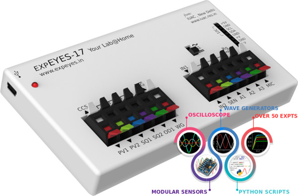
• Constant Current Source(CSS) : the constant current source can be switched ON and OFF under software control. The load resistor should be less than 3k for this current source.

• Programmable Voltage : Software controllable power supply -5V to +5V range.The resolution is 12 bits ( ~2.5 mV step size)

• Square Wave Generator SQ1 : 0 to 5 volts square wave. Frequency from 4Hz to 100kHz. The duty cycle of the output is programmable. Setting frequency to 0Hz will make the output HIGH and setting it to -1 will make it 0 Volts. SQR1 output has a 100Ω series resistor inside, so it is safe to directly connect LEDs

• Square Wave Generator SQ2 : Output swings from 0 to 5 volts and frequency can be varied from 4Hz to 100kHz. The duty cycle of the output is programmable. SQR2 is not available when WG is active.

• Digital Output (OD1) : The voltage at OD1 can be set to 0 or 5 volts using software.

• Sine/Triangular Wave WG : Frequency can be varied from 1Hz to 5kHz. The peak value of the amplitude can be set to 3 volts, 1.65 volts or 150 mV. Shape of the waqveform output is programmable, using the GUI sine or triangular can be selected. WG bar is converted into WG.

• Capacitance meter IN1 : Capacitance connected between IN1 and ground can be measured. It works better for low capacitance values, upto 10 nanoFarads but it is possible to measure in micro farad range also.

• Frequency Counter IN2: : Capable of measuring frequencies upto several Mega Hertz.

• Resistive Sensor Input(SEN) : This is mainly for sensors like Light Dependent Resistors,Thermistors,Photo-transistors etc.. It is internally connected to 3.3 volts through a 5.1kΩ resistor.

• ±16V Analog Inputs, A1 & A2 : Can measure voltage within ±16 volts range. Range can be selected from .5V to 16V fullscale. Sampling rate up to 1MSPS/Channel, giving the functionality of a low frequency oscilloscope. Both have an input impedance of 1MΩ.

• ±3.3V Analog Input A3 : Can measure voltage within ±3.3 volts range. The input can be amplified by connecting a resistor from Rg to ground, gain -1 + (Rg/10000). The input impedance of A3 is 10MΩ.

• Microphone Input MIC : A condenser microphone can be connected to this terminal and the output can be captured.

• 12C Sensor Interface : The four connections(+5V, Ground,SCL and SDA) of the 8 terminal berg strip supports 12C sensors. The software is capable of recognizing a large variety of I2C sensors for measuring temparature, velocity, acceleration etc.

• +/-6V / 10mA Power Supply : The VR+ and VR- are regulated power outputs. However,they can supply very little current, but good enough to power an Op-Amp.

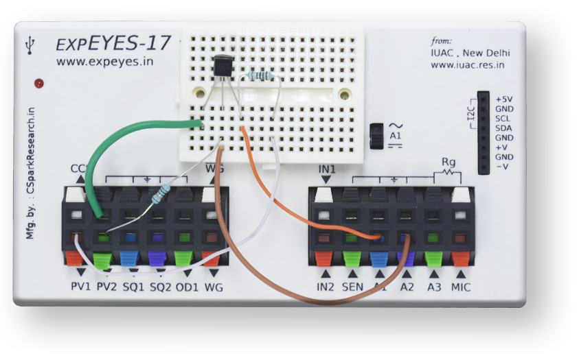
Output characteristics of an NPN transistor are being obtained in this experiment. The collector voltage is swept using the programmable voltage output, PV1, and a series 1K resistor is used to limit the current as well as to act as a shunt to measure the voltage drop across the transistor’s C & E. Base current is set via another source, PV2, and a 100k resistor. Collector and base voltages are monitored using analog inputs A1 & A2.

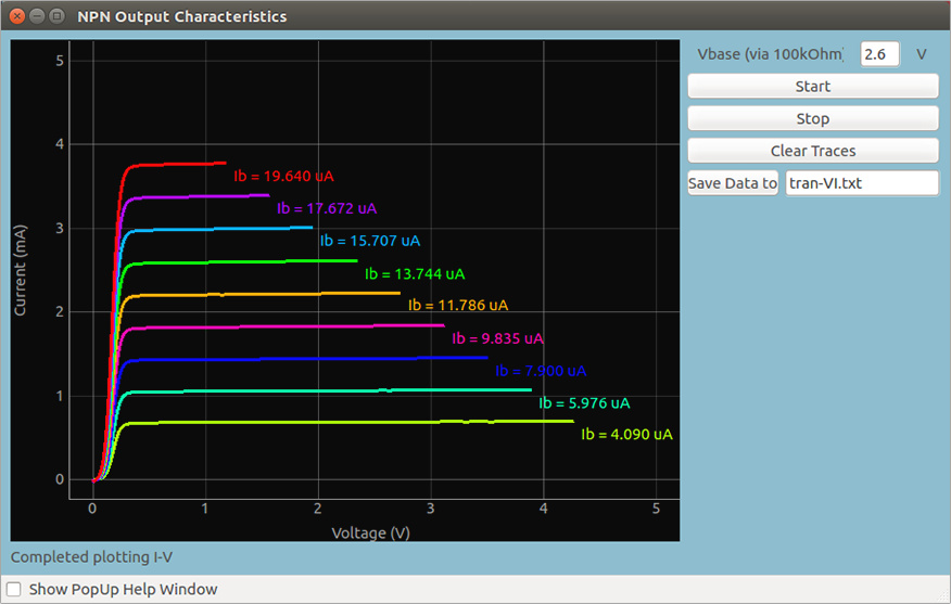
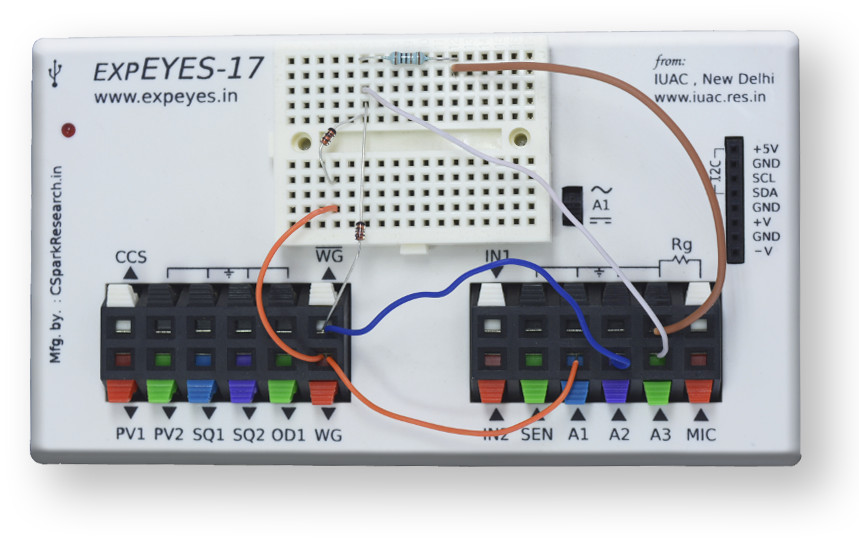
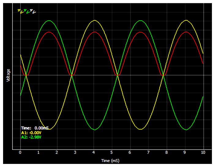
180 degree out of phase AC voltages required for the full wave rectifier are provided by WG and WG outputs. The input waveforms are monitored on A1 and A2, and the output on A3. A load resistor must be connected from A3 to ground to obtain proper output waveforms. A capacitor can be connected in parallel to the load resistor to observe the effect of filtering.

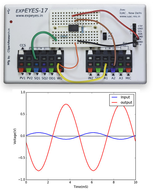
The ExpEYES hardware can be accessed via its Python library, which provides functions for operations like reading/setting voltages, measuring capacitance, time intervals etc. The example code is to study an inverting amplifier. A 200 Hz sine wave is set on WG. The channels A1 and A2 are captured and plotted, using matplotlib. Data analysis will reveal the exact gain.

from expeyes import eyes17
p = eyes17.open() 
p.set_sine(200) # 200 Hz sine wave output on WG
t,v,t2,v2 = p.capture2(500,20) #500 voltages each from A1, A2 at 20uS intervals

#Now let's use matplotlib to plot this data
from matplotlib import pyplot as plt
plt.xlabel('time (mS)') # Set the label for the x-axis . optional.
plt.ylabel('Voltage (V)') # Set the label for the x-axis . optional.
plt.plot(t,v) #input (A1)
plt.plot(t2,v2) #output of amplifier (A2)
plt.show()

Since python is a cross-platform language, running the code is possible on several Operating systems as long as the dependencies are present. For MAC, you will need to install homebrew

/usr/bin/ruby -e "$(curl -fsSL https://raw.githubusercontent.com/Homebrew/install/master/install)"

Using brew, install python3, and pip

brew install python3
brew install pip

Use Pip to install python dependencies

 pip3 install pyqt5
 pip3 install PyQtWebEngine
 pip3 install scipy
 pip3 install pyqtgraph
 pip3 install pyserial    

now, run main.py from the eyes17 source code zip. The output should resemble:

 Qt version: 5.13.0; Python version: 3.7.3 (v3.7.3:ef4ec6ed12, Mar 25 2019, 16:52:21) 
 [Clang 6.0 (clang-600.0.57)]
 Darwin-17.3.0-x86_64-i386-64bit