Full-Wave Rectification

Introduction

Full wave rectifiers enable generation of a DC signal from two out of phase AC signals.

Quick Start

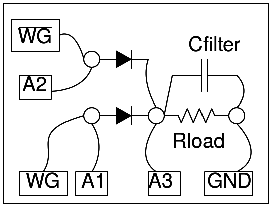
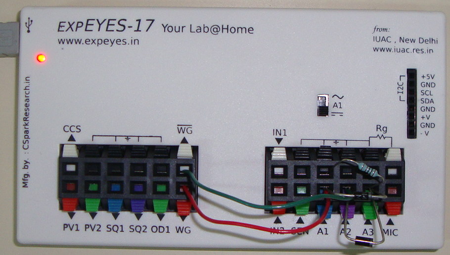
The implementation of full wave rectifier requires two AC waveforms, having 180 degree phase difference. Generally it is done using a transformer with center tap. We are using the WG and WG bar outputs for the same. WG is monitored by oscilloscope channel A1 and WG bar on A2. The rectified output is connected to A3. The observed waveform will be a bit noisy without the load resistor, connecting a 1k resistor gives a clean rectified waveform. The voltage drop across the diode is clearly visible. Connect different values of capacitors to view the filtering effect.

Screenshot of the UI

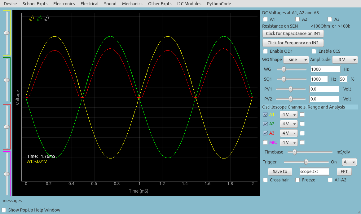
Screen shot of the oscilloscope program showing input and output of full wave rectifier. 1N4148 diode at 1000Hz and 1kOhm load resistor.

Filtering with a 1uF Capacitor

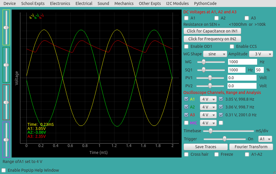
Output with R = 1kOhm and C = 1uF is shown below. It can be seen that the frequency of ripple in the case of full wave rectifier is double the frequency of the input.

Exercises

• Use a different type of diode such as a red LED for one of the input waveforms. What do you observe in the output?

Write Python Code

This experiment can also be done by running this Python Code.

#Python code to study a halfware rectifier
import eyes17.eyes
p = eyes17.eyes.open()

from pylab import *

p.set_sine(200)
t,v, t1,v1, t2, v2 = p.capture3(500, 20)   # captures A1, A2, and A3

xlabel('Time(mS)')
ylabel('Voltage(V)')
plot([0,10], [0,0], 'black')
ylim([-4,4])
plot(t,v,linewidth = 2, color = 'blue')
plot(t1, v1, linewidth = 2, color = 'red')
plot(t2,v2,linewidth = 2, color = 'green')
show()